Dangerous Accessible Space / Expected Pass Completion

Dangerous accessible space (DAS) is a flavor of EPV (expected possession value) based on physical pass simulations. For every frame where a player is in possession, the model simulates multiple ground passes of that player with different speeds and angles, such that all possible directions are covered. Then it calculates the likelihood that each player can intercept a given pass at every position along its simulated trajectory. This likelihood can then be weighted by some measure of goal threat, aggregated by team, and integrated across the pitch to give a numerical value, describing the amount of dangerous space that is accessible in the current situation.

The formula to calculate the probability to intercept or receive the ball along a pass trajectory for a given player \(r\) boils down to:

\[\frac{dP_r(t)}{dt} = P_0(t)a_r(t)\]

Where \(\frac{dP_r(t)}{dt}\) is the probability density that player \(r\) intercepts the ball at time \(t\) along the pass trajectory, \(P_0(t)\) is the probability that the ball has not been intercepted yet until time \(t\) and \(a_r(t)\) is the transition rate from \(P_0(t)\) (not intercepted) to \(P_r(t)\) (intercepted by \(r\)). The calculation of \(a_r(t)\) is based on the difference between the arrival time of a player and the ball like this:

\[a_r(t) = \frac{1}{1 + e^{b_0 + b_1(T_r(t) - t)}}\frac{1}{\sigma(v_B(t))}\]

Where \(b_0\) and \(b_1\) are parameters, \(T_r(t)\) is the arrival time of the player, \(t\) is the arrival time of the ball and \(\sigma(v_B(t))\) is a function that gives the model an additional factor that is dependent on the ball speed \(v_B(t)\) to take into account that the ability to intercept varies with the speed of the ball. Essentially, this means that the earlier a player arrives relative the ball, the higher the transition rate \(a_r(t)\) (and, accordingly, the interception probability density \(\frac{dP_r(t)}{dt}\)).

The other half of the formula, \(P_0(t)\), is calculated based on the integral of the transition rates of all players up until time \(t\). Intuitively, if a lot of players had high interception rates in the past, \(P_0(t)\) will be small and diminish all \(\frac{dP_r(t)}{dt}\) values further down the trajectory. In other words, the likelihood of interception is low if the pass has likely been intercepted before, even if the current interception rate is high.

\[P_0(t) = e^{\int_{0}^{t}(-\sum_{r \in R}^{}a_r(\tau))d\tau}\]

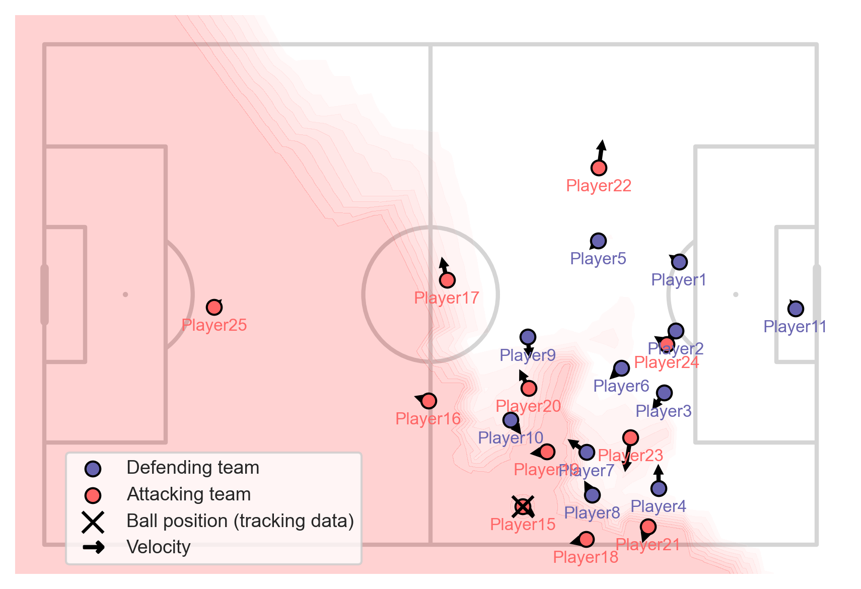
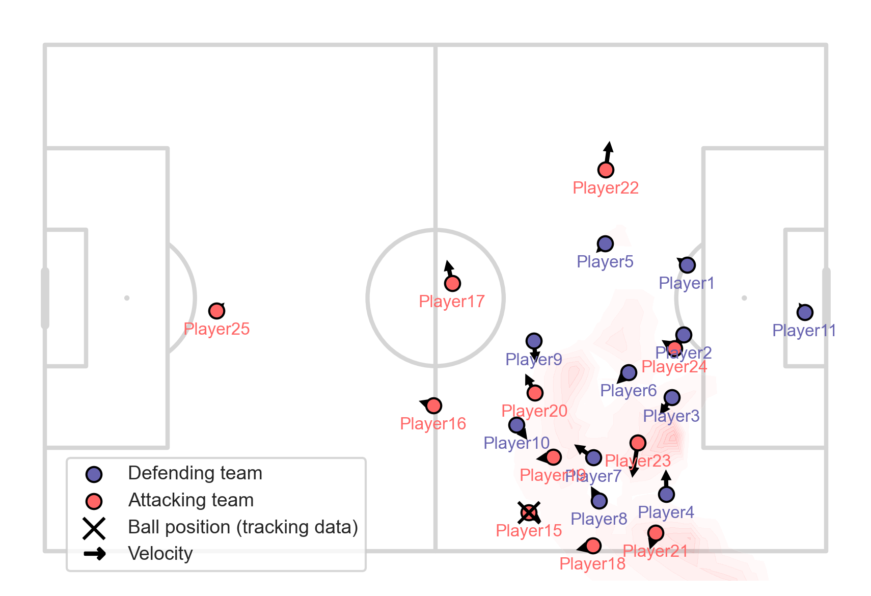
By aggregating and plotting the resulting interception probability densities \(\frac{dP_r(t)}{dt}\) spatially, we obtain the accessible space field (top image) of a team. If we add a notion of value like Expected Goals we obtain dangerous accessible space (bottom image) whose area integral serves as our final metric, DAS.

This is the gist of DAS and the physical pass simulations behind it. More details and explanations can be found in the publication of the model by Bischofberger and Baca (2025)\(^1\) and the corresponding repository\(^2\).

In databallpy, we can use the add_dangerous_accessible_space method to access team-level DAS for every frame of tracking data.

Note

The add_dangerous_accessible_space relies in the accessible-space package. You can install it with databallpy via pip install 'databallpy[accessible-space]' or simply install the package via pip install 'accessible-space>=2.0.13'

---

\(^1\) Bischofberger, J., & Baca, A. (2025). Dangerous accessible space: A unified model of space and value in team sports [Preprint]. Research Square. https://doi.org/10.21203/rs.3.rs-6932689/v1

\(^2\) jonas-bischofberger/accessible-space

from databallpy import get_open_game
import os

game = get_open_game(provider="metrica")
game.tracking_data.add_velocity(game.get_column_ids() + ["ball"], filter_type="savitzky_golay")

game.tracking_data.add_individual_player_possession()
game.synchronise_tracking_and_event_data()
game.tracking_data.add_team_possession(game.event_data, game.home_team_id)

# Add mask as argument since it can take minutes to compute it for the full match
    mask = (~pd.isnull(game.tracking_data["player_possession"])) & (game.tracking_data.index <= 1300)
game.tracking_data.add_dangerous_accessible_space(mask)

print(game.tracking_data[
    ["period_id", "frame", "team_possession", "event_id", "dangerous_accessible_space"]
].dropna()
)

	period_id	frame	team_possession	event_id	dangerous_accessible_space
365	1	366	home	-999	0.137242
366	1	367	home	-999	0.135923
367	1	368	home	-999	0.135279
368	1	369	home	-999	0.135522
369	1	370	home	-999	0.135579

Plotting DAS of both teams in a line graph highlights how the possession phases of the teams unfold during the game.

import matplotlib.pyplot as plt

df = game.tracking_data[game.tracking_data["frame"] < 1300].copy()  # Example slice

plt.figure()
plt.xlabel("Frame")
plt.ylabel("Dangerous Accessible Space [m^2]")
for team in game.tracking_data["team_possession"].dropna().unique():
    dfx = df.copy()
    i_team_possession = dfx["team_possession"] == team
    dfx.loc[~i_team_possession, "dangerous_accessible_space"] = (
        0.0  # set DAS to 0 while the opponent or no one controls the ball
    )
    dfx["dangerous_accessible_space"] = dfx["dangerous_accessible_space"].interpolate(method="linear")
    plt.plot(dfx["frame"].to_numpy(), dfx["dangerous_accessible_space"].to_numpy(), label=f"{team}")

plt.legend()
plt.show()

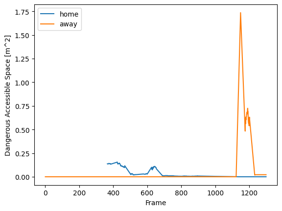
The plot shows a relatively harmless attack by the home team in the beginning, followed by a short period of danger from the away team, possibly through a ball win or a set piece.

Aggregated DAS for each team gives us a summary of their threat during the match. In the table, we can see that the home team had higher total DAS values while the away team had higher DAS values on average, pointing to a style of play more focused on counterattacking or set pieces.

dfx[dfx["dangerous_accessible_space"] > 1.5]

	frame	ball_x	ball_y	ball_z	ball_status	team_possession	home_11_x	home_11_y	home_1_x	home_1_y	...	away_32_vx	away_32_vy	away_33_vx	away_33_vy	away_34_vx	away_34_vy	away_35_vx	away_35_vy	ball_vx	ball_vy
1145	1146	-15.62820	28.45528	NaN	alive	away	-41.35425	4.78040	-25.41315	32.14564	...	NaN	NaN	NaN	NaN	NaN	NaN	NaN	NaN	-7.39	-7.61
1146	1147	-15.90540	28.16832	NaN	alive	away	-41.37525	4.79128	-25.43940	32.13612	...	NaN	NaN	NaN	NaN	NaN	NaN	NaN	NaN	-7.27	-7.50
1147	1148	-16.18155	27.88068	NaN	alive	away	-41.39835	4.80216	-25.46250	32.11572	...	NaN	NaN	NaN	NaN	NaN	NaN	NaN	NaN	-5.05	-5.55
1148	1149	-16.45770	27.59372	NaN	alive	away	-41.41935	4.81236	-25.48035	32.09668	...	NaN	NaN	NaN	NaN	NaN	NaN	NaN	NaN	-1.40	-2.32
1149	1150	-16.33170	27.66104	NaN	alive	away	-41.44455	4.82936	-25.49505	32.07832	...	NaN	NaN	NaN	NaN	NaN	NaN	NaN	NaN	2.50	1.11
1150	1151	-16.10490	27.81812	NaN	alive	away	-41.47185	4.84568	-25.50975	32.06064	...	NaN	NaN	NaN	NaN	NaN	NaN	NaN	NaN	5.43	3.70
1151	1152	-15.87810	27.97452	NaN	alive	away	-41.49810	4.86132	-25.51815	32.04228	...	NaN	NaN	NaN	NaN	NaN	NaN	NaN	NaN	6.21	4.39
1152	1153	-15.65130	28.13092	NaN	alive	away	-41.52435	4.87492	-25.52340	32.01032	...	NaN	NaN	NaN	NaN	NaN	NaN	NaN	NaN	5.79	4.02
1153	1154	-15.42450	28.28800	NaN	alive	away	-41.55060	4.88716	-25.52550	31.97632	...	NaN	NaN	NaN	NaN	NaN	NaN	NaN	NaN	5.68	3.91

9 rows × 195 columns

dfg = game.tracking_data.groupby("team_possession").agg(
    total_das=("dangerous_accessible_space", "sum"),
    max_das=("dangerous_accessible_space", "max"),
    mean_das=("dangerous_accessible_space", "mean"),
)
dfg["total_das"] /= (
    game.tracking_data.frame_rate
)  # divide by frame rate as normalization
dfg

	total_das	max_das	mean_das
team_possession
away	0.720706	1.736167	0.600588
home	0.558041	0.155625	0.046349

Internally, databallpy calls functions from the accessible-space package. That package supports additional analyses, for example, you can obtain player-level DAS values as follows:

import accessible_space

df_long = game.tracking_data[game.tracking_data["frame"].between(1140, 1160)].to_long_format()
df_long["team"] = df_long["column_id"].str[:4]

res = accessible_space.get_individual_dangerous_accessible_space(
    df_long,
    frame_col="frame",
    period_col="period_id",
    player_col="column_id",
    team_col="team",
    x_col="x",
    y_col="y",
    vx_col="vx",
    vy_col="vy",
    team_in_possession_col="team_possession",
    player_in_possession_col="player_possession",
)
df_long["AS_player"] = res.player_acc_space
df_long["DAS_player"] = res.player_das
df_long[
    ["frame", "column_id", "team", "team_possession", "AS_player", "DAS_player"]
].dropna().drop_duplicates().head(20)

Simulating passes:   0%|          | 0/1 [00:00<?, ?chunk/s]

Simulating passes: 100%|██████████| 1/1 [00:00<00:00,  1.56chunk/s]

Simulating passes: 100%|██████████| 1/1 [00:00<00:00,  1.56chunk/s]

	frame	column_id	team	team_possession	AS_player	DAS_player
21	1140	home_11	home	away	67.155876	8.689408
22	1141	home_11	home	away	54.307008	6.984953
23	1142	home_11	home	away	54.993992	6.576622
24	1143	home_11	home	away	66.006631	7.728522
25	1144	home_11	home	away	102.832008	13.799198
26	1145	home_11	home	away	113.179576	15.534433
27	1146	home_11	home	away	115.190684	19.714193
28	1147	home_11	home	away	144.758538	23.057570
29	1148	home_11	home	away	136.798579	16.665600
30	1149	home_11	home	away	141.729641	17.156089
31	1150	home_11	home	away	140.170490	16.982194
32	1151	home_11	home	away	133.792684	16.332456
33	1152	home_11	home	away	139.991248	22.521292
34	1153	home_11	home	away	136.653623	22.112414
35	1154	home_11	home	away	117.164434	19.406009
36	1155	home_11	home	away	115.958048	19.525806
37	1156	home_11	home	away	95.710890	13.818407
38	1157	home_11	home	away	78.613482	11.524109
39	1158	home_11	home	away	67.565148	8.798689
40	1159	home_11	home	away	67.181595	9.418132

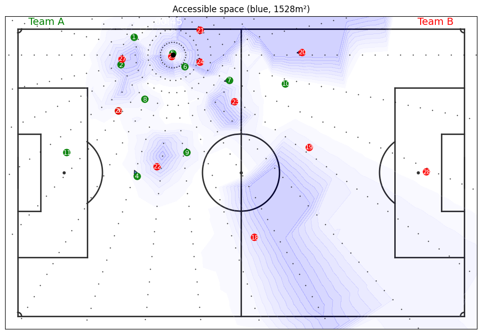
DAS can be visualized using the plot_expected_completion_surface function

from databallpy.visualize import plot_soccer_pitch, plot_tracking_data

frame_to_plot = 1148

df_tracking_frame = df_long[df_long["frame"] == frame_to_plot]

das = accessible_space.get_dangerous_accessible_space(
    df_tracking_frame,
    frame_col="frame",
    period_col="period_id",
    player_col="column_id",
    team_col="team",
    x_col="x",
    y_col="y",
    vx_col="vx",
    vy_col="vy",
    team_in_possession_col="team_possession",
    player_in_possession_col="player_possession",
)

fig, ax = plot_soccer_pitch(pitch_color="white")
fig, ax = plot_tracking_data(
    game,
    game.tracking_data[game.tracking_data["frame"] == frame_to_plot].index[0],
    fig=fig,
    ax=ax,
    title=f"Accessible space (blue, {das.acc_space.iloc[0]:.0f}m²)",
    add_velocities=True,
)

fig = accessible_space.plot_expected_completion_surface(
    das.simulation_result,  # AS
    frame_index=0,
    color="blue",
)

fig, ax = plot_soccer_pitch(pitch_color="white")
fig, ax = plot_tracking_data(
    game,
    game.tracking_data[game.tracking_data["frame"] == frame_to_plot].index[0],
    fig=fig,
    ax=ax,
    title=f"Dangerous accessible space (red, {das.das.iloc[0]:.3f}m²)",
    add_velocities=True,
)
fig = accessible_space.plot_expected_completion_surface(
    das.dangerous_result,  # DAS
    frame_index=0,
    color="red",
    plot_gridpoints=False
)

Simulating passes:   0%|          | 0/1 [00:00<?, ?chunk/s]

Simulating passes: 100%|██████████| 1/1 [00:00<00:00,  3.06chunk/s]

Simulating passes: 100%|██████████| 1/1 [00:00<00:00,  3.05chunk/s]

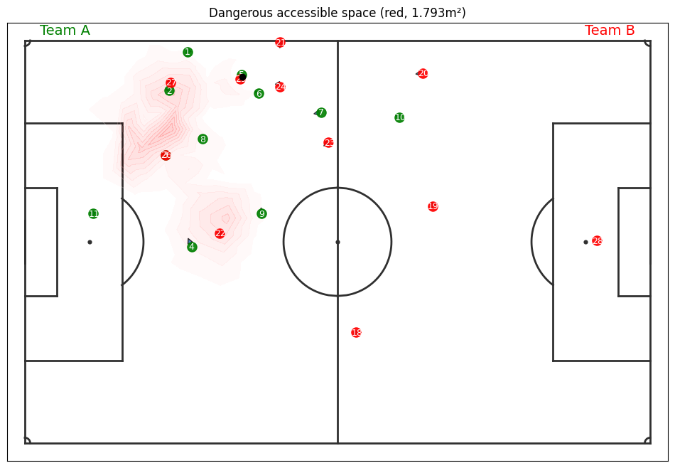
This is the moment of the high danger moment for the away team we plotted over time earlier. The striker (red 26) is at the exact same location of the defender and is therefore onside, but barely visible in the plot. If the away team is able to get the ball to him, the away team has high chances of getting ball possession at a dangerous location on the pitch, hence dangerous accessible space.

If you look at it, you might want to add some extra filters, for example, only determine the dangerous accessible space when the player is not pressured too much (have you seen the pressure feature in databallpy yet?)

For more information and excelent docs on the feature, please seethe Github repository of accessible-space.\(^2\)